Comparing conditions with replicates#
The guide goes through the tests diffsvg offers for two conditions with biological replicates, and how to read and check their results. It uses the Legnini et al. (2023) organoids: 88 genes, 4 organoids in which SHH was induced and 4 controls, with the cells of highest SHH expression as the anchor.
With 4 replicates per condition, only genes with strong effects pass a correction for testing 88 genes. Read the per-gene results as a ranked list of candidates, and use gene sets for calls about pathways.
# One BLAS thread per process; set before numpy is imported.
import os

for var in ("OMP_NUM_THREADS", "OPENBLAS_NUM_THREADS", "MKL_NUM_THREADS", "NUMEXPR_NUM_THREADS"):
    os.environ[var] = "1"

import numpy as np
import pandas as pd
import scanpy as sc
import squidpy as sq

import diffsvg as dvg

N_WORKERS = int(os.environ.get("DIFFSVG_WORKERS", 4))
LAYER = "log1p_norm"
1. Distances and replicates#
The anchor is the top 1% of SHH expression over all cells, and the setup is the same as in diffsvg in 10 minutes.
The anchor means different things in the two conditions. In control organoids, the anchor cells are a few cells with endogenous SHH. In the SHH organoids, SHH is expressed widely, so most anchor cells come from them. Differences in shape therefore mix the effect of SHH with the different meaning of “distance to the anchor”, and single-gene results need that caveat.
The 17 sections come from 8 organoids, and sections of the same organoid are not independent. bin_obs(..., sample="organoid") therefore treats each organoid as one replicate. The section slide1_A2-2 has no anchor cells, so it drops out.
adata = dvg.datasets.legnini23()  # downloads about 90 MB once, then reads from the cache

shh = sc.get.obs_df(adata, "SHH")["SHH"].to_numpy()
adata.obs["SHH+"] = (shh > np.percentile(shh, 99)).astype(str)

sq.tl.var_by_distance(
    adata, cluster_key="SHH+", groups="True", library_key="sample", covariates=["condition", "organoid"]
)
design = adata.obsm["design_matrix"]
design["organoid"] = design["organoid"].astype(str)
design.groupby("organoid", observed=True)["condition"].first().value_counts()
condition
Ctrl    4
SHH     4
Name: count, dtype: int64
dvg.pp.bin_obs(adata, anchor="True", condition="condition", layer=LAYER, sample="organoid")
setup = dvg.tl.setup_model(adata)
2. Shape, level and slope tests#
The model fits one curve of expression against distance per gene and condition, plus one random curve per organoid. Each test compares the two condition curves over the anchor support, the distances where both conditions have cells. Pick the test that matches your question before you look at the results:
test="parallel"(shape) asks whether the curves differ by more than a shift up or down.test="level"asks whether one curve is higher on average.test="slope"asks whether the gap between the curves grows or shrinks with distance.
The conditions are compared as SHH minus Ctrl, in sorted order of the labels. Each test is corrected for multiple testing over the genes (Benjamini-Hochberg, columns ending in _pval_adj), not over the three tests. With replicates, tau defaults to 0, so any difference counts; set tau to ignore differences smaller than that. If the cells cover only part of the distance range, e.g. a cell type in some cortical layers, fit_model warns; then use two_stage=True, which fits one curve per replicate and compares those curves.
results = {}
for test in ("level", "slope"):
    stats, _curves, _params = dvg.tl.fit_model(
        adata, setup, test=test, n_workers=N_WORKERS, progressbar=False, inplace=False
    )
    results[test] = stats

dvg.tl.fit_model(adata, setup, test="parallel", n_workers=N_WORKERS, progressbar=False)
results["parallel"] = adata.varm["dsvg_stats"]

pd.DataFrame(
    {
        test: {
            "p < 0.05": int((stats[f"{test}_pval"] < 0.05).sum()),
            "FDR < 0.05": int((stats[f"{test}_pval_adj"] < 0.05).sum()),
        }
        for test, stats in results.items()
    }
)
| level | slope | parallel | |
|---|---|---|---|
| p < 0.05 | 20 | 9 | 18 |
| FDR < 0.05 | 11 | 0 | 6 |
The level test finds the most genes, and no gene passes FDR for the slope test. The shape test ranks the genes by how much the gap between the curves changes beyond a constant shift. shape_diff measures that change in log-expression units over the distance range; for a gap that changes linearly it equals the change in slope. slope_diff is the slope of the gap, SHH minus Ctrl.
shape = results["parallel"].sort_values("parallel_pval")
shape[["shape_diff", "slope_diff", "parallel_pval", "parallel_pval_adj"]].head(10)
| shape_diff | slope_diff | parallel_pval | parallel_pval_adj | |
|---|---|---|---|---|
| FOXA2 | 0.325483 | 0.198719 | 9.390106e-07 | 0.000083 |
| HHIP | 1.417356 | 0.976790 | 1.204555e-04 | 0.005300 |
| PAX7 | 1.269618 | -0.996571 | 2.614018e-04 | 0.007668 |
| NEUROG2 | 1.017012 | 0.573022 | 5.412339e-04 | 0.010921 |
| GLI1 | 1.231383 | 1.036409 | 6.205072e-04 | 0.010921 |
| TBP | 0.440008 | -0.377586 | 1.932708e-03 | 0.028346 |
| FOXA1 | 0.135870 | 0.078187 | 4.075397e-03 | 0.051234 |
| Circ.RMST | 0.960115 | -0.779381 | 7.489264e-03 | 0.082195 |
| DBX2 | 1.011231 | 0.621912 | 8.406322e-03 | 0.082195 |
| PTCH1 | 1.051677 | 0.264435 | 2.171768e-02 | 0.191116 |
The top genes are SHH targets (FOXA2, HHIP, GLI1), the dorsal gene PAX7 and the proneural gene NEUROG2. TBP, a housekeeping gene, is also among the hits. A change in a housekeeping gene can come from differences in cell composition or normalisation between the conditions, so check such genes before you trust a whole list.
The level test finds the genes whose overall expression changes. The SHH-repressed genes PAX7, IRX3 and GLI3 go down, and the ventral genes NKX6.1 and NKX6.2, the neuronal gene NEUROD1 and the motor neuron marker CHAT go up, which is the ventral shift expected from SHH. Some hits have small effects, e.g. BMP4 with a level_diff of about -0.1 and BCL11B with about -0.01 log units. With tau = 0 significance doesn’t mean a relevant effect size, so sort by effect size as well.
level = results["level"].sort_values("level_pval")
level[["level_diff", "level_pval", "level_pval_adj"]].head(10)
| level_diff | level_pval | level_pval_adj | |
|---|---|---|---|
| gene | |||
| PAX7 | -2.151143 | 0.000022 | 0.001977 |
| IRX3 | -1.363535 | 0.000047 | 0.002075 |
| BMP4 | -0.097084 | 0.000397 | 0.011658 |
| GLI3 | -0.712198 | 0.000767 | 0.016882 |
| BCL11B | -0.009320 | 0.001765 | 0.025727 |
| NKX6.2 | 0.549647 | 0.001821 | 0.025727 |
| NEUROD1 | 0.406592 | 0.002046 | 0.025727 |
| NKX6.1 | 1.883516 | 0.003328 | 0.036414 |
| Circ.RMST | -1.273850 | 0.003741 | 0.036414 |
| CHAT | 0.178724 | 0.004138 | 0.036414 |
3. Curves and volcano plot#
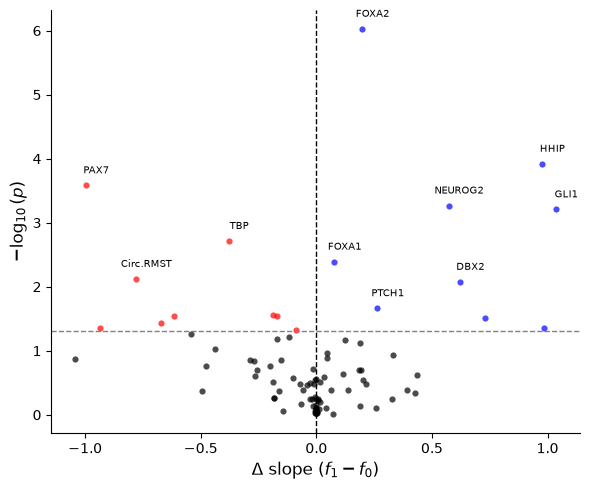
The volcano plot shows the slope of the gap between the curves against the significance of the shape test. Blue genes have an SHH minus Ctrl difference that increases with the distance from the anchor, and red genes one that decreases. Genes are coloured when their unadjusted p-value is below 0.05, the dashed line; use parallel_pval_adj for calls.
dvg.pl.plot_volcano(results["parallel"], n_label=10, figsize=(6, 5));
The curves show the posterior mean expression per condition with a 94% credible band. FOXA2 and HHIP are highest in the control organoids close to the anchor and fall within the first fifth of the distance, so the controls have a small ventral domain around their few SHH cells. In the SHH organoids these genes are low and nearly flat, so the gap between the conditions is most negative at the anchor and the slope difference is positive. PAX7, which SHH represses, is almost absent from the SHH organoids, while in the controls it rises away from the anchor. NEUROG2 is higher in the SHH organoids away from the anchor.
dvg.pl.plot_prediction_curve(adata, gene=list(shape.index[:4]));

4. Gene sets#
tl.gene_set_test summarises each organoid by one level and one slope per gene and asks whether the genes of a set change together between the conditions. It uses a rotation test, which keeps the correlation between genes and treats each organoid as one replicate. The test is self-contained: a set with a few strongly changed genes is significant even if the rest don’t change. method="ulm" asks instead whether the set changes more than the other genes (see the method page).
The sets below are SHH targets, induced by SHH, and SHH-repressed genes (class I genes of the neural tube). Any gene list or decoupler network works as a set.
genes = set(adata.var_names)
gene_sets = {
    "SHH targets": [g for g in ["GLI1", "PTCH1", "PTCH2", "HHIP", "FOXA2", "NKX2-2", "NKX6.1", "NKX6.2", "OLIG2", "NKX2-1"] if g in genes],
    "SHH-repressed": [g for g in ["PAX7", "PAX6", "PAX3", "IRX3", "MSX1", "MSX2", "DBX1", "DBX2", "GLI3", "WNT1"] if g in genes],
}  # fmt: skip
for name, members in gene_sets.items():
    print(f"{name}: {', '.join(members)}")
dvg.tl.gene_set_test(setup, gene_sets)
SHH targets: GLI1, PTCH1, HHIP, FOXA2, NKX6.1, NKX6.2, OLIG2
SHH-repressed: PAX7, PAX6, IRX3, MSX2, DBX1, DBX2, GLI3
| summary | set | size | mean_t | pval_up | pval_down | pval_mixed | pval | pval_adj | |
|---|---|---|---|---|---|---|---|---|---|
| 0 | level | SHH-repressed | 7 | -8.670715 | 1.0000 | 0.0001 | 0.0001 | 0.0002 | 0.0004 |
| 1 | level | SHH targets | 7 | 4.095945 | 0.0002 | 0.9999 | 0.0004 | 0.0004 | 0.0004 |
| 2 | slope | SHH targets | 7 | 2.719620 | 0.0039 | 0.9962 | 0.0072 | 0.0078 | 0.0156 |
| 3 | slope | SHH-repressed | 7 | -0.198673 | 0.6405 | 0.3596 | 0.0068 | 0.7192 | 0.7192 |
pval tests a common change up or down, and pval_mixed a change in either direction; the API page of gene_set_test describes all columns. In the level summary, SHH targets go up and SHH-repressed genes go down in the SHH organoids. In the slope summary, SHH targets have a positive slope difference, which is the lost gradient seen in the curves. The SHH-repressed genes have no common slope change (pval), but their slopes change in both directions (pval_mixed). Several genes in these sets already pass on their own; the set test is most useful when the single genes don’t.
5. Check with a random split#
If the organoids are split into two groups at random, no gene truly differs between the groups. The split below puts 2 SHH and 2 control organoids in each group, so the real effect cancels out, although it still adds to the variation between replicates within each group. A test with exact p-values would put about 5% of the genes, here about 4, below 0.05 and rarely any gene below FDR 0.05.
organoids = design.groupby("organoid", observed=True)["condition"].first()
rng = np.random.default_rng(0)
group_a = [*rng.choice(organoids.index[organoids == "SHH"], 2, replace=False),
           *rng.choice(organoids.index[organoids == "Ctrl"], 2, replace=False)]  # fmt: skip

real_condition = design["condition"].copy()
design["condition"] = np.where(design["organoid"].isin(group_a), "A", "B")
dvg.pp.bin_obs(adata, anchor="True", condition="condition", layer=LAYER, sample="organoid")
null_stats, _, _ = dvg.tl.fit_model(
    adata, dvg.tl.setup_model(adata), test="parallel", n_workers=N_WORKERS, progressbar=False, inplace=False
)
design["condition"] = real_condition  # restore the real conditions
print(f"random split: {(null_stats['parallel_pval'] < 0.05).sum()} genes at p < 0.05, "
      f"{(null_stats['parallel_pval_adj'] < 0.05).sum()} at FDR < 0.05")  # fmt: skip
random split: 0 genes at p < 0.05, 0 at FDR < 0.05
No gene is below p < 0.05, against the expected 4. With 4 organoids per condition the p-values are therefore conservative, which means few false hits at some cost in power. The method page summarises all 18 such splits.
Summary#
Pass the biological replicate as
sample, not the section. With 3 or 4 replicates per condition, expect only strong effects to pass FDR, so rank genes by the tests and their effect sizes and use gene sets for pathways.With one sample per condition, see Data without replicates.